Introduction
This is an Earth Engine <> TensorFlow demonstration notebook. Specifically, this notebook shows:
- Exporting training/testing data from Earth Engine in TFRecord format.
- Preparing the data for use in a TensorFlow model.
- Training and validating a simple model (Keras
Sequentialneural network) in TensorFlow. - Making predictions on image data exported from Earth Engine in TFRecord format.
- Ingesting classified image data to Earth Engine in TFRecord format.
!pip install earthengine-api
from google.colab import auth

auth.authenticate_user()
!earthengine authenticate
# Import the Earth Engine API and initialize it.
import ee
ee.Initialize()

# Test the earthengine command by getting help on upload.
!earthengine upload image -h
import tensorflow as tf

tf.enable_eager_execution()
print(tf.__version__)
import folium
print(folium.__version__)

# Define the URL format used for Earth Engine generated map tiles.
EE_TILES = 'https://earthengine.googleapis.com/map/{mapid}/{{z}}/{{x}}/{{y}}?token={token}'
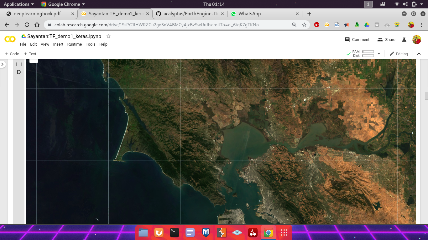
Prepare Landsat 8 imagery
First, make a cloud-masked median composite of Landsat 8 surface reflectance imagery from 2018. Check the composite by visualizing with folium.
# Use these bands for prediction.
bands = ['B2', 'B3', 'B4', 'B5', 'B6', 'B7']
# Use Landsat 8 surface reflectance data.
l8sr = ee.ImageCollection('LANDSAT/LC08/C01/T1_SR')

# Cloud masking function.
def maskL8sr(image):
  cloudShadowBitMask = ee.Number(2).pow(3).int()
  cloudsBitMask = ee.Number(2).pow(5).int()
  qa = image.select('pixel_qa')
  mask = qa.bitwiseAnd(cloudShadowBitMask).eq(0).And(
    qa.bitwiseAnd(cloudsBitMask).eq(0))
  return image.updateMask(mask).select(bands).divide(10000)

# The image input data is a 2018 cloud-masked median composite.
image = l8sr.filterDate('2018-01-01', '2018-12-31').map(maskL8sr).median()

# Use folium to visualize the imagery.
mapid = image.getMapId({'bands': ['B4', 'B3', 'B2'], 'min': 0, 'max': 0.3})
map = folium.Map(location=[38., -122.5])
folium.TileLayer(
    tiles=EE_TILES.format(**mapid),
    attr='Google Earth Engine',
    overlay=True,
    name='median composite',
  ).add_to(map)
map.add_child(folium.LayerControl())
map
Add pixel values of the composite to labeled points.
Some training labels have already been collected for you. Load the labeled points from an existing Earth Engine asset. Each point in this table has a property called landcover that stores the label, encoded as an integer. Here we overlay the points on imagery to get predictor variables along with labels.
# Change the following two lines to use your own training data.
labels = ee.FeatureCollection('projects/google/demo_landcover_labels')
label = 'landcover'

# Sample the image at the points and add a random column.
sample = image.sampleRegions(
  collection=labels, properties=[label], scale=30).randomColumn()

# Partition the sample approximately 70-30.
training = sample.filter(ee.Filter.lt('random', 0.7))
testing = sample.filter(ee.Filter.gte('random', 0.7))

from pprint import pprint

# Print the first couple points to verify.
pprint({'training': training.first().getInfo()})
pprint({'testing': testing.first().getInfo()})
Export the training and testing data
Now that there's training and testing data in Earth Engine and you've inspected a couple examples to ensure that the information you need is present, it's time to materialize the datasets in a place where the TensorFlow model has access to them. You can do that by exporting the training and testing datasets to tables in TFRecord format (learn more about TFRecord format) in a Cloud Storage bucket (learn more about creating Cloud Storage buckets). Note that you need to have write access to the Cloud Storage bucket where the files will be output.
# REPLACE WITH YOUR BUCKET!
outputBucket = 'diversion-nextera'

# Make sure the bucket exists.
print('Found Cloud Storage bucket.' if tf.gfile.Exists('gs://' + outputBucket)
    else 'Output Cloud Storage bucket does not exist.')
# Start the tasks.
trainingTask.start()
testingTask.start()
Monitor task progress
You can see all your Earth Engine tasks by listing them. It's also useful to repeatedly poll a task so you know when it's done. Here we can do that because this is a relatively quick export. Be careful when doing this with large exports because it will block the notebook from running other cells until this one completes.
# Print all tasks.
print(ee.batch.Task.list())

# Poll the training task until it's done.
import time
while trainingTask.active():
  print('Polling for task (id: {}).'.format(trainingTask.id))
  time.sleep(5)
print('Done with training export.')
fileNameSuffix = '.gz'
trainFilePath = 'gs://' + outputBucket + '/' + trainFilePrefix + fileNameSuffix
testFilePath = 'gs://' + outputBucket + '/' + testFilePrefix + fileNameSuffix

print('Found training file.' if tf.gfile.Exists(trainFilePath)
    else 'No training file found.')
print('Found testing file.' if tf.gfile.Exists(testFilePath)
    else 'No testing file found.')
Export the imagery
You can also export imagery using TFRecord format. Specifically, export whatever imagery you want to be classified by the trained model into the output Cloud Storage bucket.
imageFilePrefix = 'Image_pixel_demo_'

# Specify patch and file dimensions.
imageExportFormatOptions = {
  'patchDimensions': [256, 256],
  'maxFileSize': 104857600,
  'compressed': True
}

# Export imagery in this region.
exportRegion = ee.Geometry.Rectangle([-122.7, 37.3, -121.8, 38.00])

# Setup the task.
imageTask = ee.batch.Export.image.toCloudStorage(
  image=image,
  description='Image Export',
  fileNamePrefix=imageFilePrefix,
  bucket=outputBucket,
  scale=30,
  fileFormat='TFRecord',
  region=exportRegion.toGeoJSON()['coordinates'],
  formatOptions=imageExportFormatOptions,
)
Monitor task progress
Before making predictions, we need the image export to finish, so block until it does. This might take a few minutes...
while imageTask.active():
  print('Polling for task (id: {}).'.format(imageTask.id))
  time.sleep(5)
print('Done with image export.')
Data preparation and pre-processing
Read data from the TFRecord file into a tf.data.Dataset. Pre-process the dataset to get it into a suitable format for input to the model.
Read into a tf.data.Dataset
Here we are going to read a file in Cloud Storage into a tf.data.Dataset. (these TensorFlow docs explain more about reading data into a Dataset). Check that you can read examples from the file. The purpose here is to ensure that we can read from the file without an error. The actual content is not necessarily human readable.
# Create a dataset from the TFRecord file in Cloud Storage.
trainDataset = tf.data.TFRecordDataset(trainFilePath, compression_type='GZIP')
# Print the first record to check.
print(iter(trainDataset).next())
Define the structure of your data
For parsing the exported TFRecord files, featuresDict is a mapping between feature names (recall that featureNames contains the band and label names) and float32 tf.io.FixedLenFeature objects. This mapping is necessary for telling TensorFlow how to read data in a TFRecord file into tensors. Specifically, all numeric data exported from Earth Engine is exported as float32.
(Note: features in the TensorFlow context (i.e. feature.proto) are not to be confused with Earth Engine features (i.e. ee.Feature), where the former is a protocol message type for serialized data input to the model and the latter is a geometry-based geographic data structure.)
# List of fixed-length features, all of which are float32.
columns = [
  tf.io.FixedLenFeature(shape=[1], dtype=tf.float32) for k in featureNames
]

# Dictionary with names as keys, features as values.
featuresDict = dict(zip(featureNames, columns))

pprint(featuresDict)
Parse the dataset
Now we need to make a parsing function for the data in the TFRecord files. The data comes in flattened 2D arrays per record and we want to use the first part of the array for input to the model and the last element of the array as the class label. The parsing function reads data from a serialized Example proto (i.e. example.proto) into a dictionary in which the keys are the feature names and the values are the tensors storing the value of the features for that example. (Learn more about parsing Example protocol buffer messages).
def parse_tfrecord(example_proto):
  """The parsing function.

  Read a serialized example into the structure defined by featuresDict.

  Args:
    example_proto: a serialized Example.

  Returns:
    A tuple of the predictors dictionary and the label, cast to an `int32`.
  """
  parsed_features = tf.io.parse_single_example(example_proto, featuresDict)
  labels = parsed_features.pop(label)
  return parsed_features, tf.cast(labels, tf.int32)

# Map the function over the dataset.
parsedDataset = trainDataset.map(parse_tfrecord, num_parallel_calls=5)

# Print the first parsed record to check.
pprint(iter(parsedDataset).next())
Note that each record of the parsed dataset contains a tuple. The first element of the tuple is a dictionary with bands for keys and the numeric value of the bands for values. The second element of the tuple is a class label.
def normalizedDifference(a, b):
  """Compute normalized difference of two inputs.

  Compute (a - b) / (a + b).  If the denomenator is zero, add a small delta.

  Args:
    a: an input tensor with shape=[1]
    b: an input tensor with shape=[1]

  Returns:
    The normalized difference as a tensor.
  """
  nd = (a - b) / (a + b)
  nd_inf = (a - b) / (a + b + 0.000001)
  return tf.where(tf.is_finite(nd), nd, nd_inf)

def addNDVI(features, label):
  """Add NDVI to the dataset.
  Args:
    features: a dictionary of input tensors keyed by feature name.
    label: the target label

  Returns:
    A tuple of the input dictionary with an NDVI tensor added and the label.
  """
  features['NDVI'] = normalizedDifference(features['B5'], features['B4'])
  return features, label
Model setup
The basic workflow for classification in TensorFlow is:
- Create the model.
- Train the model (i.e.
fit()). - Use the trained model for inference (i.e.
predict()).
Here we'll create a Sequential neural network model using Keras. This simple model is inspired by examples in:
Note that the model used here is purely for demonstration purposes and hasn't gone through any performance tuning.
Create the Keras model
Before we create the model, there's still a wee bit of pre-processing to get the data into the right input shape and a format that can be used with cross-entropy loss. Specifically, Keras expects a list of inputs and a one-hot vector for the class. (See the Keras loss function docs, the TensorFlow categorical identity docs and the tf.one_hot docs for details).
Here we will use a simple neural network model with a 64 node hidden layer, a dropout layer and an output layer. Once the dataset has been prepared, define the model, compile it, fit it to the training data. See the Keras Sequential model guide for more details.
from tensorflow import keras

# How many classes there are in the model.
nClasses = 3

# Add NDVI.
inputDataset = parsedDataset.map(addNDVI)

# Keras requires inputs as a tuple.  Note that the inputs must be in the
# right shape.  Also note that to use the categorical_crossentropy loss,
# the label needs to be turned into a one-hot vector.
def toTuple(dict, label):
  return tf.transpose(list(dict.values())), tf.one_hot(indices=label, depth=nClasses)

# Repeat the input dataset as many times as necessary in batches of 10.
inputDataset = inputDataset.map(toTuple).repeat().batch(10)

# Define the layers in the model.
model = tf.keras.models.Sequential([
  tf.keras.layers.Dense(64, activation=tf.nn.relu),
  tf.keras.layers.Dropout(0.2),
  tf.keras.layers.Dense(nClasses, activation=tf.nn.softmax)
])

# Compile the model with the specified loss function.
model.compile(optimizer=tf.train.AdamOptimizer(),
              loss='categorical_crossentropy',
              metrics=['accuracy'])

# Fit the model to the training data.
# Don't forget to specify `steps_per_epoch` when calling `fit` on a dataset.
model.fit(x=inputDataset, epochs=3, steps_per_epoch=100)
Check model accuracy on the test set
Now that we have a trained model, we can evaluate it using the test dataset. To do that, read and prepare the test dataset in the same way as the training dataset. Here we specify a batch sie of 1 so that each example in the test set is used exactly once to compute model accuracy. For model steps, just specify a number larger than the test dataset size (ignore the warning).
testDataset = (
  tf.data.TFRecordDataset(testFilePath, compression_type='GZIP')
    .map(parse_tfrecord, num_parallel_calls=5)
    .map(addNDVI)
    .map(toTuple)
    .batch(1)
)

model.evaluate(testDataset, steps=100)
Use the trained model to classify an image from Earth Engine
Now it's time to classify the image that was exported from Earth Engine. If the exported image is large, it will be split into multiple TFRecord files in its destination folder. There will also be a JSON sidecar file called "the mixer" that describes the format and georeferencing of the image. Here we will find the image files and the mixer file, getting some info out of the mixer that will be useful during model inference.
Find the image files and JSON mixer file in Cloud Storage
Use gsutil to locate the files of interest in the output Cloud Storage bucket. Check to make sure your image export task finished before running the following.
# Get a list of all the files in the output bucket.
filesList = !gsutil ls 'gs://'{outputBucket}
# Get only the files generated by the image export.
exportFilesList = [s for s in filesList if imageFilePrefix in s]

# Get the list of image files and the JSON mixer file.
imageFilesList = []
jsonFile = None
for f in exportFilesList:
  if f.endswith('.tfrecord.gz'):
    imageFilesList.append(f)
  elif f.endswith('.json'):
    jsonFile = f

# Make sure the files are in the right order.
imageFilesList.sort()

pprint(imageFilesList)
print(jsonFile)
Read the JSON mixer file
The mixer contains metadata and georeferencing information for the exported patches, each of which is in a different file. Read the mixer to get some information needed for prediction.
import json

# Load the contents of the mixer file to a JSON object.
jsonText = !gsutil cat {jsonFile}
# Get a single string w/ newlines from the IPython.utils.text.SList
mixer = json.loads(jsonText.nlstr)
pprint(mixer)
# Get relevant info from the JSON mixer file.
PATCH_WIDTH = mixer['patchDimensions'][0]
PATCH_HEIGHT = mixer['patchDimensions'][1]
PATCHES = mixer['totalPatches']
PATCH_DIMENSIONS_FLAT = [PATCH_WIDTH * PATCH_HEIGHT, 1]

# Note that the tensors are in the shape of a patch, one patch for each band.
imageColumns = [
  tf.FixedLenFeature(shape=PATCH_DIMENSIONS_FLAT, dtype=tf.float32)
    for k in bands
]

# Parsing dictionary.
imageFeaturesDict = dict(zip(bands, imageColumns))

# Note that you can make one dataset from many files by specifying a list.
imageDataset = tf.data.TFRecordDataset(imageFilesList, compression_type='GZIP')

# Parsing function.
def parse_image(example_proto):
  return tf.parse_single_example(example_proto, imageFeaturesDict)

# Parse the data into tensors, one long tensor per patch.
imageDataset = imageDataset.map(parse_image, num_parallel_calls=5)

# Break our long tensors into many little ones.
imageDataset = imageDataset.flat_map(
  lambda features: tf.data.Dataset.from_tensor_slices(features)
)

# Add additional features (NDVI).
imageDataset = imageDataset.map(
  # Add NDVI to a feature that doesn't have a label.
  lambda features: addNDVI(features, None)[0]
)

# Turn the dictionary in each record into a tuple with a dummy label.
imageDataset = imageDataset.map(
  # Add a dummy target (-1), with a value that is obviously ridiculous.
  # This is because the model expects a tuple of (inputs, label).
  lambda dataDict: (tf.transpose(list(dataDict.values())), tf.constant(-1))
)

# Turn each patch into a batch.
imageDataset = imageDataset.batch(PATCH_WIDTH * PATCH_HEIGHT)
Generate predictions for the image pixels
To get predictions in each pixel, run the image dataset through the trained model using model.predict(). Print the first prediction to see that the output is a list of the three class probabilities for each pixel. Running all predictions might take a while.
# Run prediction in batches, with as many steps as there are patches.
predictions = model.predict(imageDataset, steps=PATCHES, verbose=1)

# Note that the predictions come as a numpy array.  Check the first one.
print(predictions[0])
Write the predictions to a TFRecord file
Now that there's a list of class probabilities in predictions, it's time to write them back into a file, optionally including a class label which is simply the index of the maximum probability. We'll write directly from TensorFlow to a file in the output Cloud Storage bucket.
Iterate over the list, compute class label and write the class and the probabilities in patches. Specifically, we need to write the pixels into the file as patches in the same order they came out. The records are written as serialized tf.train.Example protos. This might take a while.
outputImageFile = 'gs://' + outputBucket + '/Classified_pixel_demo.TFRecord'
print('Writing to file ' + outputImageFile)
# Instantiate the writer.
writer = tf.python_io.TFRecordWriter(outputImageFile)

# Every patch-worth of predictions we'll dump an example into the output
# file with a single feature that holds our predictions. Since our predictions
# are already in the order of the exported data, the patches we create here
# will also be in the right order.
patch = [[], [], [], []]
curPatch = 1
for prediction in predictions:
  patch[0].append(tf.argmax(prediction, 1))
  patch[1].append(prediction[0][0])
  patch[2].append(prediction[0][1])
  patch[3].append(prediction[0][2])
  # Once we've seen a patches-worth of class_ids...
  if (len(patch[0]) == PATCH_WIDTH * PATCH_HEIGHT):
    print('Done with patch ' + str(curPatch) + ' of ' + str(PATCHES) + '...')
    # Create an example
    example = tf.train.Example(
      features=tf.train.Features(
        feature={
          'prediction': tf.train.Feature(
              int64_list=tf.train.Int64List(
                  value=patch[0])),
          'bareProb': tf.train.Feature(
              float_list=tf.train.FloatList(
                  value=patch[1])),
          'vegProb': tf.train.Feature(
              float_list=tf.train.FloatList(
                  value=patch[2])),
          'waterProb': tf.train.Feature(
              float_list=tf.train.FloatList(
                  value=patch[3])),
        }
      )
    )
    # Write the example to the file and clear our patch array so it's ready for
    # another batch of class ids
    writer.write(example.SerializeToString())
    patch = [[], [], [], []]
    curPatch += 1

writer.close()
Upload the classifications to an Earth Engine asset
Verify the existence of the predictions file
At this stage, there should be a predictions TFRecord file sitting in the output Cloud Storage bucket. Use the gsutil command to verify that the predictions image (and associated mixer JSON) exist and have non-zero size.
!gsutil ls -l {outputImageFile}
Upload the classified image to Earth Engine
Upload the image to Earth Engine directly from the Cloud Storage bucket with the earthengine command. Provide both the image TFRecord file and the JSON file as arguments to earthengine upload.
# REPLACE WITH YOUR USERNAME:
USER_NAME = 'sayantandas30011998'
outputAssetID = 'users/' + USER_NAME + '/Classified_pixel_demo'
print('Writing to ' + outputAssetID)
# Start the upload
### --no-use_cloud_api.
!earthengine --no-use_cloud_api upload image --asset_id={outputAssetID} {outputImageFile} {jsonFile}
Check the status of the asset ingestion
You can also use the Earth Engine API to check the status of your asset upload. It might take a while. The upload of the image is an asset ingestion task.
ee.batch.Task.list()
View the ingested asset
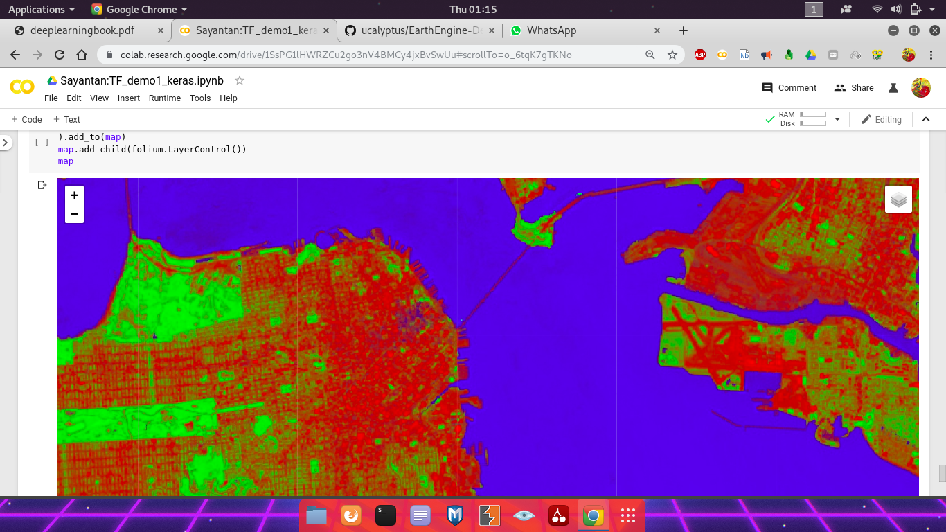
Display the vector of class probabilities as an RGB image with colors corresponding to the probability of bare, vegetation, water in a pixel. Also display the winning class using the same color palette.
predictionsImage = ee.Image(outputAssetID)

predictionVis = {
  'bands': 'prediction',
  'min': 0,
  'max': 2,
  'palette': ['red', 'green', 'blue']
}
probabilityVis = {'bands': ['bareProb', 'vegProb', 'waterProb']}

predictionMapid = predictionsImage.getMapId(predictionVis)
probabilityMapid = predictionsImage.getMapId(probabilityVis)

map = folium.Map(location=[38., -122.5])
folium.TileLayer(
  tiles=EE_TILES.format(**predictionMapid),
  attr='Google Earth Engine',
  overlay=True,
  name='prediction',
).add_to(map)
folium.TileLayer(
  tiles=EE_TILES.format(**probabilityMapid),
  attr='Google Earth Engine',
  overlay=True,
  name='probability',
).add_to(map)
map.add_child(folium.LayerControl())
map